How To Create A Heat Map In Excel - 10 Simple Steps

What Is A Heatmap?

A graphical presentation of a matrix, where each cell coloured differently and each colour has a different significance is called a heatmap. It can be used for various industries and to depict any number of different data sets, and was originally used for presenting financial data.

 

Today heatmap are used to present weather patterns, voting trends, electrical circuits’ temperature, etc. The cells colors can be either manually updated if numbers change, or dynamically updated according to the new numbers.

How To Create A Heatmap In Excel

First create an Excel Table

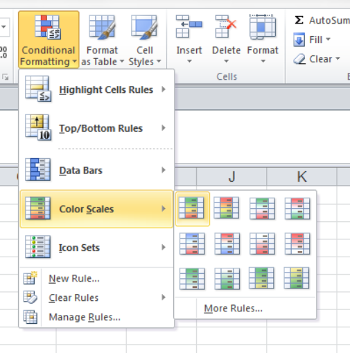
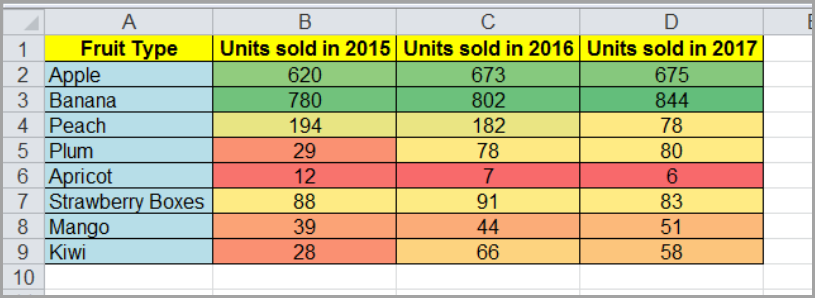
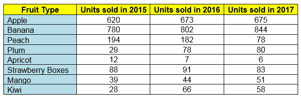
First create an excel table with the relevant columns and rows, and insert the numerical numbers into the tables’ cells. The following example presents a table with different fruit types and their unit sales from 2015, 2016 and 2017. Now choose all the cells which contain a number, and click on “Conditional Formatting -> Colour Scales” in the “Home” tab. The following menu will appear – see above picture.

Conditional Formatting Using Color Scales

Choose one of the nine available pre-set options. Each option has a different coloring scheme, and the top left possibility will colour the higher numbers in green, the middle ones in orange (middle = up to the 50th percentile) and the low ones in red. Select the “More Rules…” option and the following menu will appear 

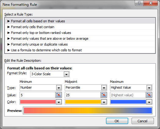
In the top half of the menu it is possible to choose the rule type. For example: the top choice allows the user to set a colouring scheme which is dependent on the value of the numbers in the table. The bottom half allows the user to change the parameters by which the cells will be coloured. For example in the “Format Style” drop down menu it is possible to choose “3-colour scale”, and then change the colour of the lower / middle/ / higher numbers, the middle percentile percentage, If the minimum / maximum will be the lowest / highest number in the table or a set number and see a preview of the scheme.

The menu below depicts a scheme in which the minimum value of the numbers is 5, the middle numbers are up to the 25th percentile, and the maximum numbers are according to the highest value in the table and are coloured blue. The higher the numbers, the darker shade of blue their cell will be. Same for the low numbers: the lower they are the redder they will be. The closer the number is to the 25th percentile, the more orange they will be. Clicking on OK in the above menu will close it, and a new menu will appear –

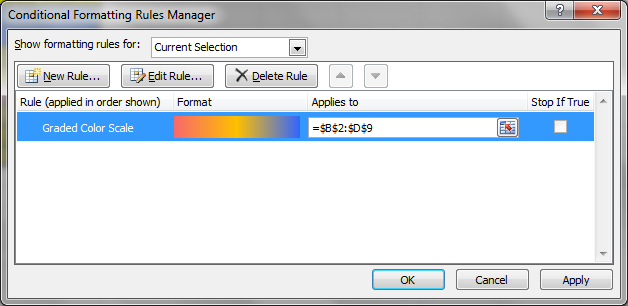
In this menu it is possible to see the colouring format, which cells it applies to and if there are any other colouring schemes in the Excel spreadsheet. Ticking the “Stop If True” checkbox will result in the next rule not to be used, in case there are more than 1 rules. Clicking “OK” will result in the rule(s) being used on the table, and the cells being coloured according to the outlined scheme.

Conditional Formatting using Icon Sets
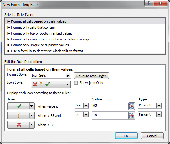
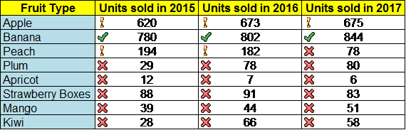
Another option is to choose the “Icon Sets” in the “Format Style”, and then choose any set in the “Icon Style” drop down menu. The menu below will result in the following colouring scheme –

• Any value in the 85th percentile and up will have a green √ next to it.
• Any value between the 85th percentile and the 15th percentile will have an orange ! next to it.
• Any value below the 15th percentile will have a red X next to it.